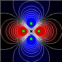
Four charged particles produce a quadrupole
electrostatic potential.
An Introduction to Computer Simulation Methods
Chapter 10 Examples: Electrodynamics
We compute the electric fields due to static and moving charges, describe methods for computing the
electric potential in boundary value problems, and solve Maxwell's equations numerically.
The following EJS models are described in Chapter 10 of the EJS adaptation of An Introduction to Computer Simulation Methods.
-
Point Charge Electric Field: Draws a grid of vectors to show the electric field from multiple point charges. The model stores ten particle locations
but only the first n particles are visible and only these active particles are used to compute the field. Whenever a charge is added or moved, the electric
field is recomputed using a fixed relation.
- Electric Field Lines: Draws electric field lines in the vicinity of
point charges. The field line is drawn by solving an ODE in response to a mouse click.
- Laplace Equation: Uses the relaxation method to solve the boundary value problem of finding the potential V(x,y) in a charge-free
region bounded by conductors. For teaching purposes, the problem is solved using the Jacobi method but the more efficient Gauss-Seidel method is also
implemented on a disabled evolution page.
- Vector Field: Displays the vector field A=(Ax, Ay). The vector field visualization uses arrows that have the
same length but different colors. Using color rather than arrow length to represent a vector field's strength produces a more effective representation
of magnitude over a wider range of values.
- Analytic Vector Field: This model is similar to the Vector Field model except that it uses an Analytic Vector Field rather than a Vector
Field element to display the field. The analytic element is simpler to use because it accepts two strings, rather than two arrays, representing as input
and parses these strings into mathematical expressions to compute the field components.
- Scalar Field Gradient: Displays the gradient by overlaying a vector field on scalar field U(x,y). The gradient of a scalar field U(x,y) is
a vector field that points in the direction of the greatest rate of change of the scalar field. The Scalar Field Gradient Model computes this gradient
using the central difference approximation to the partial derivatives.
Download
An Introduction to Computer Simulation Methods examples are distributed as a ready-to-run (compiled) Java archive. Double clicking the
csm_ch10.jar file will run the chapter 10 examples if Java is installed. You can examine and modify the model for
these examples if you have EJS installed by right-clicking within the program and selecting "Open Ejs Model" from the pop-up menu.