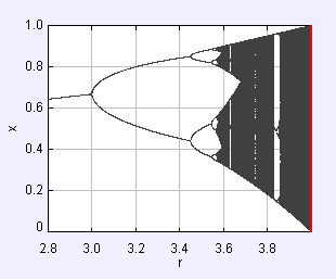
The logistic map bifurcation plot.
An Introduction to Computer Simulation Methods
Chapter 6 Examples: The Chaotic Motion of Dynamical Systems
We study the simple nonlinear deterministic models that exhibit chaotic
behavior. We will find that the use of the computer to do numerical experiments will help us gain insight into the nature of chaos.
The following EJS models are described in Chapter
6 of the EJS adaptation of An Introduction to Computer Simulation Methods.
- Iteration: The Iteration model computes a table of iterates {x0, x1, x2, x3, · · ·} using a map xn+1
= f(xn) that computes a sequence of numbers starting with a seed x0 and a control parameter r and repeatedly applying the map. The sequence of
iterates is referred to as a trajectory or an orbit.
- Logistic Bifurcation: The Bifurcation model shows the long-term iterates of the logistic map xn+1 = 4rxn(xn − 1) as a function of the control
parameter r. The model plots the iterated values xn after the initial transient behavior is discarded. If the trajectory is close to an attractor, only
those points that lie on the attractor will appear on the plot. The Bifurcation model nicely shows the forking of the possible periods of stable orbits from
1 to 2 to 4 to 8 etc. as r is increased. Each of these bifurcation points is a period-doubling bifurcation.
- Logistic Cobweb: The Logistic Cobweb model shows the behavior of the logistic map by showing a cobweb plot, a table of iterates, and a plot of
iterates. The cobweb plot consists of a diagonal (x = y) line and a curve representing y = 4rx(1 − x). Starting with an initial seed x0, the plot shows how
visually how the logistic map produces successive iterates. The cobweb spirals inward toward a stable fixed point. Period doubling produces closed loops,
and chaotic orbits show a filled area.
- Logistic Lyapunov: The Logistic Lyapunov Exponent model plots the Lyapunov exponent to shows the rate of separation of logistic map trajectories.
- Two Ball Bounce: The Two Ball Bounce model shows a two-ball collision in a constant gravitational field that is constrained to move in one
dimension above a fixed floor. Except when a collision occurs, each ball is a freely falling particle. The model also displays a Poincare map using the
velocity v1 and height y1 of the upper ball m1 at the instant that the lower ball m2 hits the floor.
Download
- Chapter 6 XML source code in a zip archive. Unzip this model in the EJS workspace.
- Chapter 6 ready to run examples in a jar file.
- Chapter 6 text in PDF format
An Introduction to Computer Simulation Methods examples are distributed as a ready-to-run (compiled) Java archive. Double clicking the
csm_ch05.jar file will run the chapter 3 examples if Java is installed. You can examine and modify the model for
these examples if you have EJS installed by right-clicking within the program and selecting "Open Ejs Model" from the pop-up menu.