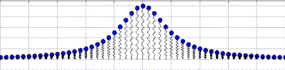
A comparison of fifty-one driven simple harmonic oscillators with differing natural frequencies.
An Introduction to Computer Simulation Methods
Chapter 4 Examples: Oscillations
We explore the behavior of oscillatory systems, including the simple harmonic oscillator, a simple
pendulum, and electrical circuits and we introduce the concept of phase space. We also show how the EJS ODE editor is used to solve arrays of differential
equations.
The following EJS models are described in Chapter 4 of the EJS adaptation of An Introduction to Computer Simulation Methods.
- SHO Solver Comparison The SHO Solver Comparison model solves the simple
harmonic oscillator (SHO) differential equation using various fixed step size solution algorithms. The simulation allows users
to change the step size and uses radio buttons to select the algorithm: Euler, Euler-Richardson, Verlet, and 4th order
Runge-Kutta. The output graph in the main window displays the analytic and numerical solution and the Data Tool can be used to
compare multiple solutions.
- Traveling Wave The Traveling Wave model plots A sin(k x + \omega t) as a
function of t. This wave function has both spatial and temporal oscillatory motion and the model shows how how to plot
such a time-varying function.
- Simple Pendulum The Simple Pendulum model solves the pendulum differential
equation using a 4th order Runge-Kutta algorithm. The model is set up and solved using polar coordinates and the view displays
the pendulum using polar coordinate axes. This model also demonstrates how to draw the pendulum using as a group of objects and
how to rotate the group.
- Driven SHO Comparison The Driven SHO Comparison model displays fifty-one
oscillators with different natural frequencies driven by an external force. The oscillator mass increases from left to right in
the multi-oscillator display and the oscillator in the center has a mass of one. All oscillators are driven with a synchronous
external sinusoidal force. The model displays each oscillator as an element of an set and the evolution workpanel for this model
shows how EJS solves arrays of differential equations.
- SHO Frequency Response The SHO Frequency Response model computes a
resonance curve by plotting the SHO steady state amplitude as a function of drive frequency. The ODE solver advances the
dynamical variables for many drive cycles using the Cash-Karp adaptive step algorithm. The simulation then computes the
amplitude of oscillation and increments the frequency in preparation for the next evolution step.
- RC Circuit The RC Circuit model simulates a resistor and a capacitor in
series with either a sinusoidal or a square wave source voltage Vs(t) and plots the time dependence of the voltage drops across
the source, the resistor, and the capacitor. The resistance, capacitance, and source frequency can be varied by the user.
- RLC Circuit The RLC Circuit model simulates a resistor, a capacitor, and
an inductor in series with either a sinusoidal or a square wave source voltage Vs(t) and plots the time dependence of the
voltage drops across the source, the resistor, and the capacitor. The resistance, capacitance, and source frequency can be
varied by the user.
- Truck Drawing The Truck Drawing model shows how to group multiple elements
so that the group can be moved, resized, and rotated as a single object.
Download
The EJS adaptation of an Introduction to Computer Simulation Methods examples are distributed as a ready-to-run (compiled) Java archive. Downloading
and then double clicking the
csm_ch04.jar file will run the chapter 4 examples if Java is installed. You can examine and modify
these examples if you have EJS installed by right-clicking within a running simulation and selecting "Open Ejs Model" from the pop-up menu.