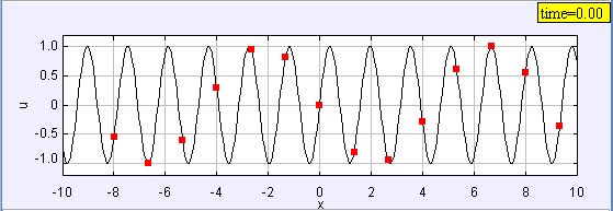
[The Wave Function Sampling Model shows how sampling affects our ability to reconstruct a function from data.]

[The Wave Function Sampling Model shows how sampling affects our ability to reconstruct a function from data.]
In order to study the relation between EJS and Java, we build time dependent function plotters. We describe common data types and we explore various user interface elements and show how to control their appearance. Finally, we show how to use a parser to input functions and how to access methods in EJS Objects.
The Wave Function Sampling Model demonstrates how function sampling affects our ability to reconstruct that function from data. This model builds on previous models by overlaying view elements to show both the original wave function and the sampled data. The function that is displayed is defined using a global string variable (fstring) that is parsed into a mathematical expression.
The Wave Function Sampling Model uses the parser inside Function Element to convert a string into a mathematical expression. The element's Input property is a string that is displayed in the graphical user interface and is passed to the internal parser. If the user enters an incorrect mathematical expression, the input field automatically turns red.
In this model the expression is a function of more than one variable.
The wave function is sampled at n points and this data is stored and displayed in a Trail Element. Unlike previous models, the trail's X and Y-Input properties are empty and the trial does not automatically collect data from the model. The Wave Function Sampling Model adds and removes data using explicit statements on a fixed relations code page.
//Fixed relations code page
double dx = (xmax-xmin)/n;                     // sample interval
double x=xmin+dx/2;                            // position
_view.trail.clear();                           // clear old data
for(int i=0; i<n; i++) {                       // loop to create new data
  double u = _view.waveFunction.evaluate(x,t); // evaluate wave function
  _view.trail.addPoint(x,u);                   // add data to trace
  x += dx;                                     // increment position
}
Methods in the trail are accessed using the Java dot operator that was introduced in the Time Dependent Function Model. The code defines and initializes local variables that are used to generate data within a loop. Old data in the trail is cleared before entering the loop and new data is added to the the trail as the loop is iterated. The new data is displayed because EJS automatically repaints the screen after fixed relations are evaluated.
The wave function is displayed using an Analytic Curve Elements and its properties are set using its inspector.
The Variable property should be set to \code{x} because it specifies the independent parameter that will be incremented. The X() and Y() properties are functions of this independent parameter and are strings that will be processed by a parser. The $x$-coordinate function is a string (literal) that does not change so we enter it as \code{"x"}. The $y$-coordinate function is a variable that does change so we enter the variable name surrounded with percent signs as explained previously. The Java Syntax property allows us to parse code expressions such as \code{Math.sin}, but it is set to \code{false} because we wish to input functions using standard mathematical notation. We could specify the number of points using the Points property, but this is unnecessary as \ejs\ automatically chooses a sufficient number of points to give a smooth curve. Minimum and Maximum properties are also not specified because we are plotting a function of $x$, and the analytic curve uses the $x$-axis minimum and maximum values as defaults.
\note{The mathematical expression parser is very powerful. Unknown symbols within an expression are automatically associated with corresponding variables in the model. If the model defines variables named \code{amp}, \code{freq}, and \code{delta}, the user can entered the expression \texttt{amp*Math.sin(freq*x + delta*t)} into the function's text field and the function correctly evaluate the expression.}
Strings are Objects representing text as a string of characters. (Read the previous sentence again.) Because text is very important when programming, Java allows us to define string objects by placing the text between quotation marks.
String hello="Hello world!";
Strings have methods and these methods are invoked using the dot operator. We can, for example, invoke the hello string to find its length.
int n= hello.length(); // hello String defined previously
Inspectors have property fields and EJS converts each property entry into an appropriate data type before it is used. The x-position of a shape, for example, should be a number so EJS converts the characters 3+5 into the number 8 before setting the shape's x-position. If the property value is a string, EJS assumes the user has entered a literal value and converts the characters into a String and adds quotation marks in the inspector field.
If a property field contains characters and if that property value is a number, EJS assumes that the characters refer to an expression that can be converted to a number. For example, if we wish to place a shape two units to the right of the xmin value, we enter xmin+2 into the x-position property. EJS find the global xmin variable in the variables table and uses its value to evaluate the expression.
There is, however, an ambiguity between a literal expression and a variable name when a property value is a string.
The following EJS models demonstrate how to plot time dependent functions in EJS. These models are listed in order of complexity.
The Wave Function Sampling Model was created by Wolfgang Christian using the Easy Java Simulations (EJS) version 4.1 authoring and modeling tool. You can examine and modify a compiled EJS model if you run the model (double click on the model's jar file), right-click within a plot, and select "Open Ejs Model" from the pop-up menu. You must, of course, have EJS installed on your computer.
Information about Ejs is available at: <http://www.um.es/fem/Ejs/> and in the OSP ComPADRE collection <http://www.compadre.org/OSP/>.