[The Evolution workpanel controls a time dependent model.]
[The Evolution workpanel controls a time dependent model.]
In order to study the relation between EJS and Java, we build time dependent function plotters. We describe common data types and we explore various user interface elements and show how to control their appearance. Finally, we show how to use a parser to input functions and how to access methods in EJS Objects.
The Time Dependent Plot Model displays the time evolution of u = sin(2*t). This simple model illustrates how EJS Elements automatically collect data when variables change. You can cut and paste portions of this model into other models as you develop your own time dependent simulations.
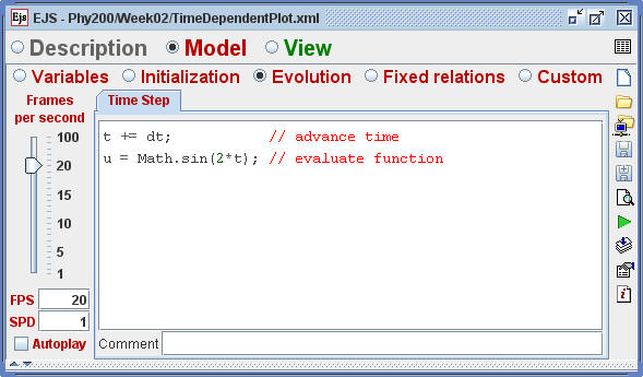
The Evolution workpanel allows us to build time-dependent models using either ordinary differential equations or Java code. We start our study of time development using a code page that plots a sinusoidal function. Open the Time Dependent Plot Model and navigate to the Evolution workpanel. Study the property fields on this panel. The frames per second (FPS) property specifies how many times per second the simulation updates (repaints) its view elements, such as graphs and tables. This simulation repaints the screen 20 times per second. The steps per display (SPD) property determines how many computations (evolution steps) are performed before each screen update. In this simulation data is generated in real time because the time step dt and the time between screen updates are equal and because the computation is performed once per screen update. The Autoplay box is unchecked on the Evolution workpanel because the user controls the time evolution using buttons.
The Time Dependent Plot Model evaluates and displays a function u = f(t) in real time by generating data at a constant (fixed) rate as shown in the screen shot. The data is generate with the following code:
t += dt;           // advance time
u = Math.sin(2*t); // evaluate function
The independent variable t and the dependent variable u are displayed in a Trace within the model's plotting panel. The t and u variables are connected (bound) to the X and Y Input properties and the Element automatically collects data from the model as these variables change during the time evolution.
| Method Name | Description |
|---|---|
| _initialize() | Executes code on the initialize workpanel followed by Fixed Relation code. |
| _isPaused() | Returns true if the evolution is not running. |
| _pause() | Pauses the evolution. |
| _play() | Begins the evolution. |
| _reset() | Resets the simulation to its initial state. |
| _view.resetTraces() | Removes the data from all trace and trail Elements. |
[Examples of predefined methods that can be used throughout a model.]
EJS automatically generates the code needed for the view (user interface) and the model contains just enough code to implement the physics. But how can we programmatically control the view without direct access to the view? For example, how can we programmatically stop a simulation when a projectile crashes into an object? EJS contains a number of predefined utility methods to perform common tasks as shown in the table. These methods can be invoked anywhere in a model. For example, we can stop the time evolution of our model after 10 time units by adding the following statement to the evolution:
if(t>=10){    // check for maximum time
  _pause();   // stop the evolution
}
A complete list of predefined and custom methods is displayed by right-clicking within a code page. Documentation is available on the EJS website.
Predefined methods are often used within action methods. Navigate to the Tree of Elements and examine the action methods for the
model's buttons. The reset button  rests the
simulation to its default state by invoking the model's _reset() method and the step button
rests the
simulation to its default state by invoking the model's _reset() method and the step button
 invokes the _step() method.
Note that the start button is a two-state button with different actions and different images depending on its state.
invokes the _step() method.
Note that the start button is a two-state button with different actions and different images depending on its state.
The following EJS models demonstrate how to plot time dependent functions in EJS. These models are listed in order of complexity.
The Time Dependent Plot model was created by Wolfgang Christian using the Easy Java Simulations (EJS) version 4.1 authoring and modeling tool. You can examine and modify a compiled EJS model if you run the model (double click on the model's jar file), right-click within a plot, and select "Open Ejs Model" from the pop-up menu. You must, of course, have EJS installed on your computer.
Information about Ejs is available at: <http://www.um.es/fem/Ejs/> and in the OSP ComPADRE collection <http://www.compadre.org/OSP/>.