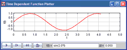
[The Time Dependent Function Model generates data using an expression parser.]

[The Time Dependent Function Model generates data using an expression parser.]
In order to study the relation between EJS and Java, we build time dependent function plotters. We describe common data types and we explore various user interface elements and show how to control their appearance. Finally, we show how to use a parser to input functions and how to access methods in EJS Objects.
The Time Dependent Function Model evaluates an arbitrary function y = f(t) at a fixed rate. Unlike the Time Dependent Plot Model, the function can be changed while the program is running. The model used the Function Element to parser and to plot a function that is represented as a string.

[Mathematical functions recognized by the Function Element parser.]
In order to build models that allow users to input functions, we need to convert a sequence of characters into a mathematical expression that can be evaluated. Code that does this conversion is known as a parser. A Function Element is an input field that accepts a string and parses it. This element is on input and output tab of the Interface palette the and is usually added to a panel. The string can be changed at any time and can contain the functions shown in the table.
EJS gives the model access to View Elements using the dot operator. We have already used this notation to evaluate trigonometric functions in the Math class and to print strings using the System class.
double y = Math.sin(x);
System.out.println("y="+y);
The first statement says: "Use the Math class to compute the sine of x and store the returned value in y." The second statement says: "Use the output in the System class to print a string." The notation to access the Function in the view is similar. In the Evolution workpanel we write:
u = _view.analyticFunction.evaluate(t); // evaluate function
This statement says: "Evaluate the mathematical expression in the view's analytic function and store the result in u."
When we design a view by selecting EJS Elements from palettes and place them in the view, we are creating Java objects in computer memory. Each object has property variables, such as color, and code that can do useful things, like compute numbers or output data. For example, the compute first point custom method uses methods in objects three times.
public void computeFirstPoint () {
  t=0;
  _view.clearData();                        // clear old data
  u = _view.analyticFunction.evaluate(t);     // compute u
  _view.trail2D.addPoint(t,u);                // add first xy-point
}
It takes time and practice to learn what each EJS Element can do but a list of methods is displayed in a drop down menu when you type an object's name in a code page. Documentation is also available on the EJS website for each Element by clicking on the information icon in top left corner of an element's inspector.
Syntax Note: Because it is possible to create many different Function Elements, we must use the name that appears in the Tree of Elements to access the object. The sine method in the Math class is different from the evaluate method in the Function Element because the sine function never changes so we can access it using the Math class name. There is only one mathematical sine function after all. Methods that can be accessed using a class name are known as static methods. Methods that can access a particular object are known as instance methods. We will come back to the distinction between static and instance methods later in the course when we create our own own objects.
The following EJS models demonstrate how to plot time dependent functions in EJS. These models are listed in order of complexity.
The Time Dependent Function Plot model was created by Wolfgang Christian using the Easy Java Simulations (EJS) version 4.1 authoring and modeling tool. You can examine and modify a compiled EJS model if you run the model (double click on the model's jar file), right-click within a plot, and select "Open Ejs Model" from the pop-up menu. You must, of course, have EJS installed on your computer.
Information about Ejs is available at: <http://www.um.es/fem/Ejs/> and in the OSP ComPADRE collection <http://www.compadre.org/OSP/>.