[User interface elements often perform actions within an EJS model.]
[User interface elements often perform actions within an EJS model.]
Our first objective will be to become familiar with the EJS modeling environment and to compile and run simple examples that demonstrate how EJS works and basic Java syntax. Students will also learn how to create a ready-to-run Java program (jar file) and how to submit EJS homework as zip files.
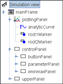
The Quadratic Equation Solver with Actions Model extends the second quadratic equation example by allowing the user to directly manipulate the quadratic equation's roots. The r1 and r2 output fields have been enabled to allow users to enter values and the blue root markers on the graph are now draggable. The model shows how a dynamic user interface (View) interacts with the underlying model.
A fixed relations code page is invoked (evaluated) automatically whenever an EJS model changes. Custom methods allow you to create code pages that are invoked explicitly. Open the Quadratic Equation Solver with Analytic Plot Model and examine the Custom workpanel in the Model. The Custom workpanel contains a single code page named Compute Coefficients with the following code:
/*
 * Computes the coefficients when the roots r1 and r2 change.
 * The quadratic coefficient a remains unchanged.
*/
public void computeCoefficients() {	// beginning of method body
  b=-a*(r1+r2);
  c=a*r1*r2;
}					// end of method body
An EJS Custom method is a subroutine that is associated with an EJS model. Method bodies usually consist of a sequence of statements to perform a computation that changes the state of the model. The compute coefficients method, for example changes the quadratic equation coefficients. This method is invoked (called) using a statement on a code page. For example, if we wish to visualize a quadratic equation with roots at x3 and x=-6, we write the following code:
r1=3.0;			// sets the value of the first root
r2=-6.0;		// sets the value of the second root
computeCoefficients();  // computes new quadratic equation coefficients
The compute coefficients method does not affect the model if it is never invoked.
Syntax note: The public qualifier in the method declaration indicates that this method can be used anywhere within the model. The void return type indicates that the method does not return a value. Later in this course we will define methods that accept input parameters and return values. A trigonometric sine method, for example, would almost certainly take an input value and return the answer and could be declared as follows:
public double sin(double angle){  	// beginning of method body
  // don't worry about the code in the body
  // you know how to use the method from the declaration
}					// end of method body
The compute coefficients method should be performed (invoked) when the user types a new coefficient into a coefficient input field. Open the model and examine the Action property on the inspector panel for the root1Field or the root2Field in the Tree of Elements. Click on the editor icon for the Action property and note that the Action is a code page with a single statement:
computeCoefficients();
When a user edits the root1Field the Input property value EJS sets the r1 variable to the new value and then executes the action code followed by fixed relation code. The fixed relation computes the r1 and r2 value and should (presumable) give the same value that the user entered into the field. This computation is unnecessary but harmless. Input actions occur infrequently extra computation that is required to insure that roots are always consistent with the coefficient values is fast.
The same paradigm applies to the circular markers. Examine the root1Marker inspector panel and study the shape's properties. The X Input property is connected (bound) to the r1 variable so that the dragging the shape affects this variable. The Y Input property is not a variable but an arithmetic expression that computes the vertical position of the shape. The On Drag action invokes the compute coefficients method when the user performs a mouse action. Fixed relations are enforced after all actions have been processed again bringing the model into a consistent state.
The quadratic equation models demonstrates that EJS modeling is quite different from programming. The physics and the mathematics of the model are described with a small amount of code and almost no code is required to create the user interface. Much of the Java programming required to produce a complete simulation is hidden from the user. The user interface is is constructed by dragging and dropping Elements onto user interface tree and the Elements are connected to the underlying model using inspector panels. This structured approach to modeling helps us understanding and see the relationship between the user interface and the model parts without coding. The modeling process is devoted to understanding and documenting the model, to experimenting with the model, and to writing about the results.
The following introductory EJS models demonstrate how to solve the quadratic equation and how to plot a function in EJS. These models are listed in order of complexity.
The Quadratic Equation models were created by Wolfgang Christian using the Easy Java Simulations (EJS) version 4.1 authoring and modeling tool. You can examine and modify a compiled EJS model if you run the program by double clicking on the model's jar file. Right-click within the running program and select "Open EJS Model" from the pop-up menu to copy the model's XML description into EJS. You must, of course, have EJS installed on your computer.
Information about EJS is available at: <http://www.um.es/fem/Ejs/> and in the OSP ComPADRE collection <http://www.compadre.org/OSP/>.