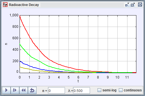
[Radioactive decay curves.]

Week 10 Notes: Random Processes

We study models that use random numbers to generate statistically predictable outcomes.  Examples include Monte Carlo methods and random walks on a lattice.  Many of the random walk models are described in Chapter 7 of An Introduction to Computer Simulation Methods.

Radioactive Decay

The EJS Radioactive Decay Model simulates the decay of a radioactive sample using discrete random events.  If the number of radioactive nuclei N is large, the rate of change of N can be approximated as a differential equation

where the decay constant λ is a positive number.   The solution to this equation is an exponential decay function.

Nuclei are, however, discrete and this continuous model fails when the number of nuclei is small.

The probability P of one nucleus decaying in a time interval Δt is

If exponent in this equation is small, this probability is approximately λΔt.

Run the model and observe the stochastic (random) behavior when the number of particles is small.  The check box switches to a semi-log graph to more clearly show the exponential nature of the decay curve.

Credits:

The Radioactive Decay Model was created by Wolfgang Christian using the Easy Java Simulations (EJS) authoring and modeling tool.  You can examine and modify a compiled EJS model if you run the program by double clicking on the model's jar file.  Right-click within the running program and select "Open EJS Model" from the pop-up menu to copy the model's XML description into EJS.  You must, of course, have EJS installed on your computer.

Information about EJS is available at: <http://www.um.es/fem/Ejs/> and in the OSP comPADRE collection <http://www.compadre.org/OSP/>.