
We study models that use random numbers to generate statistically predictable outcomes. Examples include Monte Carlo methods and random walks on a lattice. Many of the random walk models are described in Chapter 7 of An Introduction to Computer Simulation Methods.
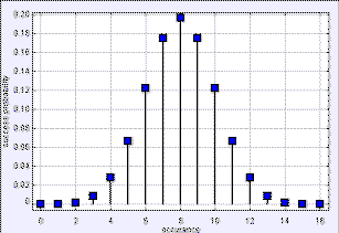
The binomial distribution is the discrete probability distribution of the number of successes in a sequence of n independent yes/no trials, each of which yields success with probability p. The Binomial Distribution Model shows the probability of k successful outcomes after n trials.
The Binomial Distribution Model is both inefficient and limited insofar as it can only compute coefficients for 20 trials before an integer overflow occurs
in the factorial computation. If you have EJS installed
(see the Credits below), disable the existing custom method code page and add a new custom method to that uses the Stirling approximation (or some other way of handling
the large values of factorials since 25! uses 26
digits: see
Computer Science wiki):
Test your new model for large numbers of trials.
The following EJS models use random numbers to generate statistically predictable outcomes.
Wikipedia: http://en.wikipedia.org/wiki/Binomial_distribution
The Binomial Distribution Model was created by Wolfgang Christian using the Easy Java Simulations (EJS) authoring and modeling tool. You can examine and modify a compiled EJS model if you run the program by double clicking on the model's jar file. Right-click within the running program and select "Open EJS Model" from the pop-up menu to copy the model's XML description into EJS. You must, of course, have EJS installed on your computer.
Information about EJS is available at: <http://www.um.es/fem/Ejs/> and in the OSP comPADRE collection <http://www.compadre.org/OSP/>.