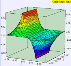
[The electric potential near two plates with fixed potential.]
We study scalar and vector fields in 2D and learn how to solve Laplace's equation using the relaxation method.
Suppose that we do not know the positions of the charges and instead know only the potential on a set of boundaries surrounding a 2D charge-free region. This information is sufficient to determine the potential V(x,y) at any point within the charge-free region. The direct method of solving for V(x,y) is based on Laplace's equation which can be expressed in Cartesian coordinates as
The problem is to find the function V(x,y) that satisfies the Laplace's equation and the specified boundary conditions. This type of problem is an example of a boundary value problem. Because analytical methods for regions of arbitrary shape do not exist, the only general approach is to use numerical methods. Laplace's equation is not a new law of physics, but can be derived from the definition of electric potential in regions of space where there is no charge.
The following EJS models demonstrate how to display two-dimensional scalar and vector fields using elements on the fields and plots tab on the EJS 2D Drawables palette.
The Laplace Equation Model was created by Wolfgang Christian using the Easy Java Simulations (EJS) version 4.1 authoring and modeling tool. The model is adapted from on Section 10.5 of An Introduction to Computer Simulation Methods by H. Gould, J. Tobochnik and W. Christian.
You can examine and modify a compiled EJS model if you run the model (double click on the model's jar file), right-click within a plot, and select "Open Ejs Model" from the pop-up menu. You must, of course, have EJS installed on your computer. Information about Ejs is available at: <http://www.um.es/fem/Ejs/> and in the OSP comPADRE collection <http://www.compadre.org/OSP/>.