
We continue our study of dynamical systems by studying systems with additional degrees of freedom.
Newton's Second Law for one-dimensional linear motion states that the acceleration is proportional to the force F applied to that object:
F = m a.
For planar rotation the Second Law states that the angular acceleration α of an object is proportional to the torque τ applied to that object:
τ = I α .
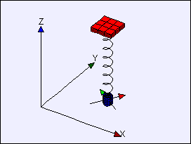
What happens if these motions are coupled? In other words, assume that translating the object produces a small torque and that rotating the object produces a small line (linear) force. This coupling occurs naturally if we suspend a mass from a coil spring. The spring tends to uncoil as it is stretched and this uncoiling produces a rotation of the mass. The Wilberforce Pendulum Model displays the resulting motion.
A Wilberforce Pendulum, named after its inventor, Lionel Robert Wilberforce, consists of a mass hanging off a spring, and is an example of a coupled oscillator system. The spring and the mass are specially designed so that energy and oscillatory motion are transferred back and forth between the up and down oscillation of the spring, and the rotational motion of the mass. Under the proper conditions, the pendulum can exhibit a curious behavior, whereby at one time, all of the movement is purely rotational and the spring is static, and at a later time, this is reversed. This back and forth transfer is periodic and can happen indefinitely (in the absence of damping forces).
The following differential equation models will be discussed in class.
Additional models may be be posted for self-study.
The Wilberforce Pendulum Model was created by Wolfgang Christian using the Easy Java Simulations (EJS) version 4.1 authoring and modeling tool. You can examine and modify a compiled EJS model if you run the model (double click on the model's jar file), right-click within a plot, and select "Open Ejs Model" from the pop-up menu. You must, of course, have EJS installed on your computer.
Information about Ejs is available at: <http://www.um.es/fem/Ejs/> and in the OSP comPADRE collection <http://www.compadre.org/OSP/>.