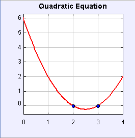
[Screen shot of quadratic function plot.]

[Screen shot of quadratic function plot.]
Our first objective will be to become familiar with the EJS modeling environment and to compile and run simple examples that demonstrate how EJS works and basic Java syntax. Students will also learn how to create a ready-to-run Java program (jar file) and how to submit EJS homework as zip files.
The Quadratic Equation with Plot Model extends our first model by adding a plot of the polynomial function. There are many ways to plot a function in EJS and this model uses a numeric approach in order to introduce loops and arrays.
Array variables are very common in science and mathematics because they allow us to refer to related values using a single variable name. In this example we use x and y array variables to store the plot data. Array elements are accessed using an integer index enclosed in square brackets following for variable name. We could, for example, assign array elements to plot a sin curve as shown in the following code fragment:
x[0]=-10.0;		// stores value in first x array element
y[0]=Math.sin(x[0]);	// stores value in first y array element
x[1]=-9.9;		// stores value in second x array element
y[1]=Math.sin(x[1]);	// stores value in second y array element
// Etc
The Quadratic Equation with Plot Model x and y data arrays are used as input for a Trace Element in the View and our x and y arrays have 500 array elements. It would be cumbersome to access every element of an array by explicitly coding every array index. Computers are well suited to perform repetitive operations and these operations are often defined using a for loop. In this model, we use a loop to compute the xy data points that display the quadratic function.
/*
 * Computes y(x)=a*x*x + b*x + c at np points and stores data points in x[] and y[] arrays.
 * The function y(x) is evaluated at np points from xmin to xmax.
*/

double xLocal=xmin;                      // independent variable
double dx=(xmax-xmin)/(np-1);            // variable increment
for(int i=0; i<np; i++){                 // set up loop
  x[i] = xLocal;                         // store independent variable in array
  y[i]=a*(xLocal+b)*xLocal+c;	         // compute function and store in array
  xLocal += dx;                          // increment independent variable
}                      			 // end of loop body
The statements in the code declares x and dx variables and assigns initial values. The third statement begins the loop. A loop typically requires the declaration and initialization of a counter variable (int i=0), a test to determine if the counter variable has reached its terminal value (i<n), and a rule for changing the counter variable (i++) after every iteration. In Java syntax, these three parts of the for loop are contained within parentheses and are separated by semicolons.
A loop executes a single statement following the loop until end of loop test is false. Matched curly braces create a code block that acts is if it were a single Java statement so that we can define complex loop bodies. In this example the body of the loop is a code block that contains three statements. The code block is executed n times and each iteration assigns a value to successive array elements x[i] and y[i].
It is customary to indent statements within a code block, such as the body of a loop, so that it can be easily identified. Java ignores indentation (whitespace), but it provides an important visual cue to the code's logical structure. You can reformat a code page to indent code by right-clicking within the code page and selecting the format option.
Note the use of the ++ increment operator for the end of loop operation rather than the equivalent expression i = i + 1. The ++ operator is common programming practice because it is compact and faster than the equivalent expression. The += operator is also a common programming idiom and is equivalent to addition followed by assignment. In other words, x0 += dx is equivalent to x0 = x0 + dx.

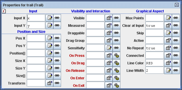
[Trail Element inspector. Most properties retain their default values.]
EJS drawing Elements are located on palettes in the View workpanel. This model uses Trail Element to display the xy data points. Double click the trail in the View of Elements to open its inspector and note that only 6 of 27 inspector fields are set. The input fields allow the Element to collect data from the model and the Clear at Input field determines if the old data should be removed when new data is obtained. The Clear at Input field is set to true because the input variable contain the entire dataset. This field is usually false if the trail is collecting single xy data points during a Time evolution.
Because property fields have reasonable default values, it is usually unnecessary to enter many values. Rest the mouse on the property label to view a descriptive "hint" right-click within the field to examine its default value. You can also click on the small information button in the upper left hand corner to obtain detailed documentation from the EJS server.
The following introductory EJS models demonstrate how to solve the quadratic equation and how to plot a function in EJS. These models are listed in order of complexity.
The Quadratic Equation models were created by Wolfgang Christian using the Easy Java Simulations (EJS) version 4.1 authoring and modeling tool. You can examine and modify a compiled EJS model if you run the program by double clicking on the model's jar file. Right-click within the running program and select "Open EJS Model" from the pop-up menu to copy the model's XML description into EJS. You must, of course, have EJS installed on your computer.
Information about EJS is available at: <http://www.um.es/fem/Ejs/> and in the OSP ComPADRE collection <http://www.compadre.org/OSP/>.